Microsoft Excel
Creating Graphs in Microsoft Excel
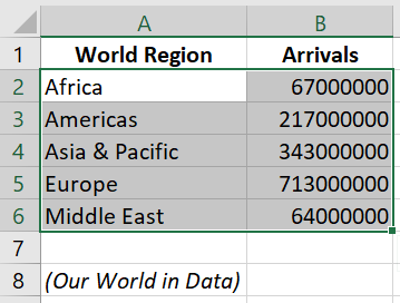
1. Check that the information and data are in columns next to each other, with no blank columns in between.

Ensure the numbers don't have any spaces e.g. 5000, not 5 000.

2. Highlight the information and data ONLY.
You can highlight the headings of each column, but sometimes the graph may not work if they are highlighted.
You can highlight the headings of each column, but sometimes the graph may not work if they are highlighted.
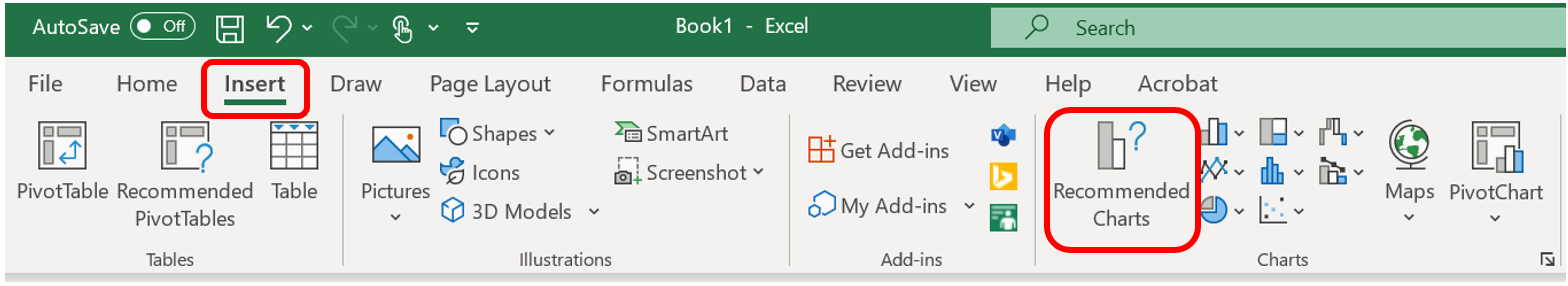
3. Click on the 'Insert' tab
4. Go to the 'Charts' section
5. Click on 'Recommended Charts'.
4. Go to the 'Charts' section
5. Click on 'Recommended Charts'.
6. Click on the 'All Charts' tab and select the most suitable type of graph to represent your data down the left hand side.
For Types of Graphs, go to this page: Types of Graphs - Geography (weebly.com).
For Types of Graphs, go to this page: Types of Graphs - Geography (weebly.com).

Editing the Graph
Chart Title
Edit the chart title by clicking on the title, deleting the word 'chart title' and writing in a suitable one for this graph. Consider what the data is communicating. Check your typing/spelling to ensure it is correct.
Other Edits
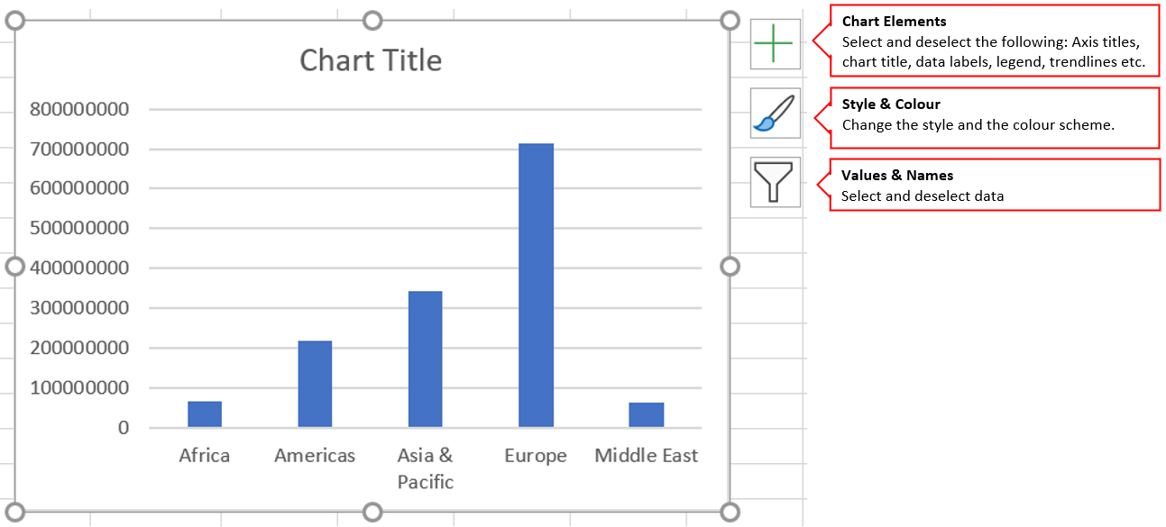
You can further edit the graph by clicking on the graph and then the icons on the right hand side.
Edit the chart title by clicking on the title, deleting the word 'chart title' and writing in a suitable one for this graph. Consider what the data is communicating. Check your typing/spelling to ensure it is correct.
Other Edits
You can further edit the graph by clicking on the graph and then the icons on the right hand side.
- Top icon 'Chart Elements' - you can select and deselect a range of features and elements for the graph. Carefully consider what is important and what is not needed.
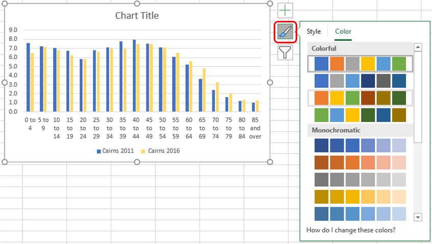
- Middle icon 'Style & Colour' - you can change the style and colour scheme. Keep it simple and clear to be able to visualise the data effectively. Avoid using dark backgrounds.
- Bottom icon 'Values & Names' - this allows you to focus on some of the data only.
Re-sizing/Moving Elements of a Graph
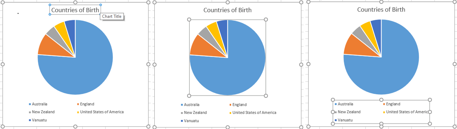
You can move and re-size elements (specific parts) of the graph by selecting them.
For example. below are examples of selecting the chart title, whole pie graph, and key.
For example. below are examples of selecting the chart title, whole pie graph, and key.
|
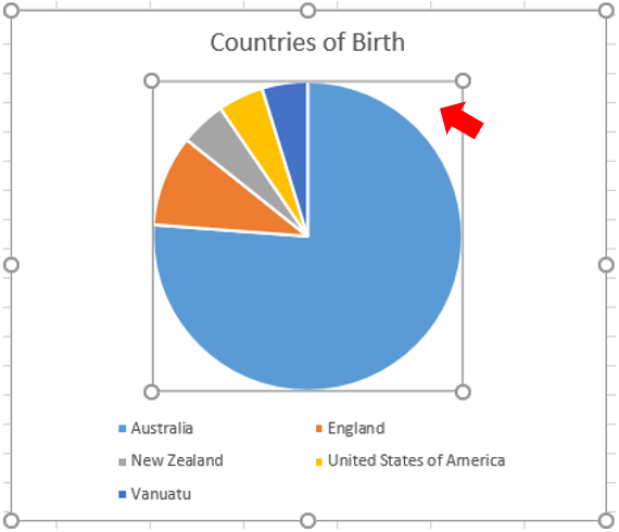
To select the whole pie graph, pretend it is a square and click on one of the corners (see red arrow)
|
To select just a slice of the pie, click on the slice (see red arrow).
You can move the slice around to emphasise it 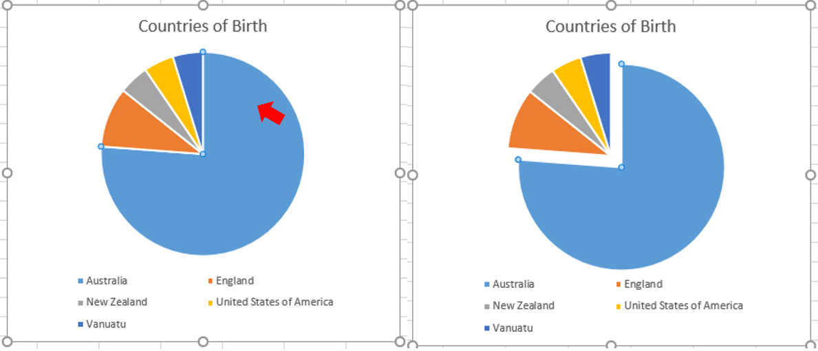
|
An example of selecting a column graph to resize it.

Axes
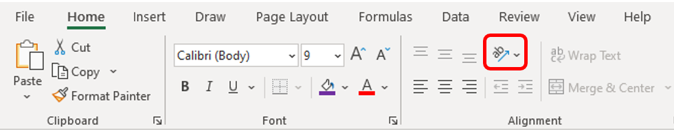
To change text direction
Changing Colours
Change the colour scheme of the graph.
Click on the whole graph > Paint brush icon > Color
Click on the whole graph > Paint brush icon > Color
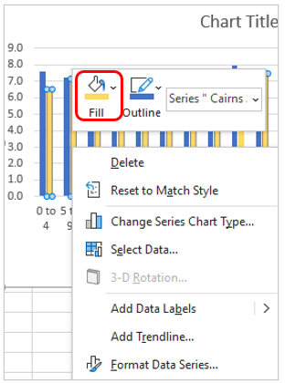
Change colours of individual parts of the graph
Right click on the part of the graph (e.g. column) and ensure all specific parts are highlighted > Fill
Right click on the part of the graph (e.g. column) and ensure all specific parts are highlighted > Fill
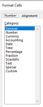
Formatting Cells
Right click on the cell > Format Cells

|
|
General - no specific format.
Number - for general display of numbers. Currency - used for monetary values. It will add a selected currency symbol before the number e.g. $. Accounting - line up the currency symbols and decimal points in the column. Date - displays data and time serial numbers as date values. Time - displays data and time serial numbers as date values. Percentage - multiply the cell value by 1-- and displays the result with a percent symbol (%). Fraction - choose how it is represented. Scientific - Text - treated as a text even when a number is in the cell. The cell is displayed exactly as entered. Special - useful for tracking list and database values. Custom - select from a range of options. |
Formulas - Adding a Formula to a Cell
- Double click on the cell to edit
- Once you have entered the formula, press enter to finalise the cell. If you click out of it, you will select another cell
SYMBOLS
Multiply *
Equal =
Divide /
Formulas - Common Formulas
CELL refers to the selected cell on Microsoft Excel e.g. B2.
Instead of a CELL, it could also be a number you type out.
Range of Cells (B2:B9) - includes all cells from B2 to B9, so B2, B3, B4 etc.
Select Cells individually (B2,B4,B7)
Instead of a CELL, it could also be a number you type out.
Range of Cells (B2:B9) - includes all cells from B2 to B9, so B2, B3, B4 etc.
Select Cells individually (B2,B4,B7)
Addition
=SUM(CELL:CELL) - best for adding up numbers over more than two cells
=(CELL+CELL) - if you just want to add the numbers of two cells together
Subtraction
=(CELL-CELL)
Multiplication
=(CELL*CELL)
Division
=(CELL/CELL)
=SUM(CELL:CELL) - best for adding up numbers over more than two cells
=(CELL+CELL) - if you just want to add the numbers of two cells together
Subtraction
=(CELL-CELL)
Multiplication
=(CELL*CELL)
Division
=(CELL/CELL)
For more formulas:
Top 30 Excel Formulas and Functions You Should Know | Simplilearn
Top 30 Excel Formulas and Functions You Should Know | Simplilearn
Formulas - Applying a Formula to All Cells
Tips for applying the formula to all cells
- Select the cell with the formula you just entered.
- Click on the bottom right hand corner (where the little green square is) and drag it down. The cells should populate with the formula.
- Alternatively, select the blank cell underneath the cell with the formula you just entered. On the Home tab, go to Fill and click on Down
Excel Shortcuts

(Excel Insider)
